Tag Archives: curve complex

Quick post: research updates of friends

18 Aug

I noticed a few papers up on arXiv last week that correspond to some old posts, so I thought I’d make a quick note that these people are still doing math research and maybe you are curious about it!

We last saw Federica Fanoni and Hugo Parlier when they explored kissing numbers, and they gave an upper bound on the number of systoles (shortest closed curves) that a surface with cusps can have.  This time they give a lower bound on the number of curves that fill such a surface.  Remember, filling means that if you cut up all the curves, you end up with a pile of disks (and disks with holes in them).  So you can check out that paper here.

Last time we saw Bill Menasco, he was working with Joan Birman and Dan Margalit to show that efficient geodesics exist in the curve complex.  This new paper up on arxiv was actually cited in that previous paper- it explains the software that a bunch of now-grad students put together with Menasco when they were undergrads in Buffalo, NY (UB and Buffalo State) during this incredible sounding undergrad research opportunity– looks like the grant is over, but how amazing was that- years of undergrads working for an entire year on real research with a seminar and a semester of preparation, and then getting to TA a differential equations class at the end of your undergraduate career.  Wow.  I’m so impressed.  I got sidetracked: the software they made calculates distances in the curve complex and the paper explains the math behind it and includes lots of pretty pictures.

My friend Jeremy did a guest post about baklava and torus knots a long time ago, and of course he’s got his own wildly popular blog.  He also has a bunch of publications up on arXiv, including one from this summer.  They’re all listed in computer science but have a bunch of (not-pure) math in them.

The paper I worked on over that summer at Tufts with Moon Duchin, her student Andrew Sánchez (note to self: I need a good looking website I should text Andrew), my old friend Matt Cordes, and graduate student superstar Turbo Ho is up on arXiv and has been submitted: it’s on random nilpotent quotients.

Moon and Andrew and others from that summer have another paper which has been accepted to a journal, it’s also about random groups and is here.  It was super cool, I saw a talk at MSRI during my graduate summer school there and John Mackay (also a coauthor on that paper) was in the audience and this result came up organically during the talk.  Pretty great!

There’s another secret project from that summer which isn’t out yet, but I just checked two of the three co-authors webpages and they had three and four papers out in 2015 (!!!)  That’s so many papers!  So I don’t know when secret project will be out but I’ll post about it when it is.

I really enjoy posting about current research in mathematics and trying to translate it into undergrad-readability, so I’ll try to continue doing so.  But this Thursday you’ll read about cinnamon buns instead.  Yum.

Efficient geodesics in the curve complex

15 Jul

I have a not-secret love affair with blogging the curve complex: I (intro), II (dead ends), III (connected).  I’m surprised I didn’t blog the surprising and cute and wonderful proof that the curve complex is hyperbolic, which came out two years ago.  Maybe I’ll do that next math post (but I have a large backlog of math I want to blog).  Anyways, I was idly scrolling through arXiv (where mathematicians put their papers before they’re published) and saw a new paper by the two who did the dead ends paper, plus a new co-author.  So I thought I’d tell you about it!

If you don’t remember or know what the curve complex is, you’d better check out that blog post I (intro) above (it is also here in case you didn’t want to reread the last paragraph).  Remember that we look at curves (loops) up to homotopy, or wriggling.  In this post we’ll also talk about arcs, which have two different endpoints (so they’re lines instead of loops), still defined up to homotopy.

The main thing we’ll be looking at in this post are geodesics, which are the shortest path between two points in a space.  There might be more than one geodesic between two spaces, like in the taxicab metric.  In fact, in the curve complex there are infinitely many geodesics between any two points.

It's easy to get metrics messed up, but the taxicab metric is pretty straightforward

It’s easy to get metrics messed up, but the taxicab metric is pretty straightforward- there are lots of geodesics between the red star and the starting point.  I guess if you’re an alien crossed with a UFO crossed with a taxi then maybe the metric is difficult (butI totally nailed portraits of UFO-taxi-aliens)

Infinity is sort of a lot, so we’ll be considering specific types of geodesics instead.  First we need a little bit more vocabulary.  Let’s say I give you an arc and a simple (doesn’t self intersect) closed curve (loop) in a surface, and you wriggle them around up to homotopy.  If you give me a drawing of the two of them, I’ll tell you that they’re in minimal position if the drawings you give me intersect the least number of times of all such drawings.

All three toruses have the same red and green homotopy classes of curves.  I just couldn't make a picture w/out a cute blushing square.

All three toruses have the same red and green homotopy classes of curves, but only the top right is in minimal position – you can homotope the red curve in the other two pictures to decrease the number of times red and green intersect.  I just couldn’t make a picture w/out a cute blushing square.

If you have three curves a, b, c all in minimal position with each other, then a reference arc for a,b,c is an arc which is in minimal position with b, and whose interior is disjoint from both and c.

Green is a reference arc for red, orange, yellow: its interior doesn't hit red or yellow, and it intersects orange once.

Green is a reference arc for red, orange, yellow: its interior doesn’t hit red or yellow, and it intersects orange once.  Notice that it starts and ends in different points, unlike the loops.  (This picture is on a torus) [Also red and yellow aren’t actually in minimal position; why not?]

Now if you give me a series of curves on a surface, I can hop over to the curve complex of that surface and see that series as a path.  If the path $latex v_0,v_1,\ldots,v_nis geodesic, then we say it is initially efficient if any choice of reference arc for v_0,v_1,v_n intersects v_1 at most n-1 times.

The geodesic v_0,v_1,\ldots,v_n is an efficient geodesic if all of these geodesics are initially efficient: (v_0,\ldots, v_n), (v_1,\ldots,v_n),\ldots,(v_{n-3},\ldots,v_n).  In this paper, Birman, Margalit, and Menasco prove that efficient geodesics always exist if v_0,v_n have distance at least three.

Note that there are a bunch of choices for reference arcs, even in the picture above, and at first glance that “bunch” looks like “infinitely many,” which sort of puts us back where we started (infinity is a lot).  Turns out that there’s only finitely many reference arcs we have to consider as long as d(v_0,v_n)\geq 3.  Remember, if you’ve got two curves that are distance three from each other, they have to fill the surface: that means if you cut along both of them, you’ll end up with a big pile of topological disks.  In this case, they take this pile and make them actual polygons with straight sides labeled by the cut curves.  A bit more topology shows that you only end up with finitely many reference arcs that matter (essentially, there’s only finitely many interesting polygons, and then there are only so many ways to draw lines across a polygon).

So the main theorem of the paper is that efficient geodesics exist.  The reason why we’d care about them is the second part of the theorem: that there are at most n^{6g-6} many curves that can appear as the first vertex in such a geodesic, which means that there are finitely many efficient geodesics between any two vertices where they exist.

Here’s the link to the paper if you feel like checking it out.

I DID NOT MAKE THIS PICTURE IT IS FROM BIRMAN, MARGALIT, MENASCO.  But look at how cool it is!!!

I DID NOT MAKE THIS PICTURE IT IS FROM BIRMAN, MARGALIT, MENASCO. But look at how cool it is!!!

Look at this picture!  The red curve and blue curve are both vertices in the curve complex, and they have distance 4 in the curve complex, and here they are on a surface!  So pretty!

If you feel like wikipedia-ing, check out one of the authors on this paper.  Birman got her Ph.D. when she was 41 and is still active today (she’s 88 and a badass and I want to be as cool as she is when I grow up).

The curve complex is connected

24 Aug

So I’ve spent my summer traveling, “baking” (see all the raw posts), and doing a little bit of math.  More specifically, I’ve been reading A Primer on Mapping Class Groups, by Benson Farb and Dan Margalit, with my friends Ellie and Mike.   Remember how I had that post introducing the curve complex? And the second one? Well, I thought we’d delve just an eensy bit deeper into that and prove something with some fun topological methods!

Sometimes math is really beautiful when mathematicians name things in a totally sensible way. A graph is connected if it’s all one piece. If you really want a fancier pants-ier definition, a graph is n-connected if, after you remove any (n-1) vertices from it, it remains just one component (you can trace a path between any two vertices). Here are examples of a disconnected, connected, and 2-connected graph:

Usually we're happier when graphs are connected.  The one on the left is being silly and contrary.

Usually we’re happier when graphs are connected. The one on the left is being silly and contrary.

Notice that the 1-connected graph is NOT 2-connected, because if you remove the red vertex and all the edges leading to it, you end up with 2 components.  Whereas in the 2-connected graph, removing any one vertex doesn’t disconnected the graph.  This was a tiny tangent, as we don’t need n-connectivity right now (who knows, we might use it in the future of this blog! There’s lots of math out there!) We’re focusing on 1-connectivity.

So we’re proving that the aforementioned curve complex is connected (there are a couple of exceptions to this, by which I mean this statement is true for almost all surfaces but there’s like 5 times when it’s not.  I’ll talk about those later). That means that if you hand me two vertices from the curve complex, I should be able to find a path between them. So, looking at our surface, that means if you hand me two closed curves x and y on a surface, I should be able to find a sequence of curves a_i such that a_0=x, a_n=y, and a_i,a_{i+1} are disjoint.

Let’s say you’re being silly and you hand me an x and y that are already disjoint. Then we’re done! Theorem proved, right?

Obviously not, because what if you hand me an x and y that aren’t disjoint? What then, you ask me?

Well, we’d better figure out a way to classify cases: I don’t have time to just stand here looking for a sequence of disjoint curves for every pair you give me. Instead, I’ll make boxes for types of pairs to live in, and then I’ll say that there always EXISTS a sequence of curves (without me explicitly finding them). If I make enough boxes to deal with ALL possible pairs of curves, and I deal with all of those boxes, then I’ve proven the theorem.

I’ve already proven the theorem for the case that you gave me two disjoint curves. We could say that they intersect zero times, or, to use some more wonderfully accurate math terminology, that x and y have intersection number 0. We write this as i(x,y)=0. For any two curves you give me, there’ll be a minimal intersection number, by which I mean none of this squiggly nonsense:

intersectionnumber

Even though I can count 5 intersection points between these two curves in the top picture, they minimally intersect just once, as you can see by straightening them out in the bottom picture.

This means that any pair of curves will live in a box labeled by its intersection number- we have “enough” boxes to deal with whatever curves you hand me. So let’s look at these boxes.

If i(x,y)=1
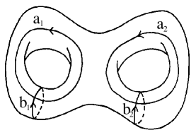
, that means there’s a neighborhood around these curves that looks like a torus with a hole on the side:

oncepncturedtorus

The “hole” connects our two curves to the rest of the surface (I didn’t draw it but it lives over on the right.

So just take the blue curve that goes around that hole in the big surface. Label that curve a. Then the path \{x, a, y\} connects x and y, with consecutive members of our sequence disjoint. So in the curve complex, there’s a path of length two between x and y.

Two boxes down, just… infinitely more to go.  But if I can manipulate any of my infinite boxes to fit into one of the two that we already know, I’ll be done.  This is sort of the gist of the principle of induction (this is a link to wikipedia). (I will make an induction post sometime).  Now suppose that i(x,y)\geq 2.

We want to reduce this to an earlier case. So let’s try to find a blue curve c with a smaller intersection number with both x and y- by the principle of induction, there’ll be a path from c to x, and one from c to y. So x and y will be connected by a path, which is exactly what we want.

surgery

To find c, we first make a parallel copy of x, which intersects y the same number of times (of course). So we pick two of these intersection points next to each other on y and redirect our parallel copy of x so it only intersects y once instead of twice, thus decreasing the intersection number. Look at the pictures to make this clear: x is the green curve, y is the red curve, and c is the blue curve. Our c will intersect with x once, and with y fewer times than i(x,y).

That’s it! Good job team! This was some hard work but hopefully a bit fun for you- we proved that the curve complex is connected, using lots of pictures and some cold, hard logic.

*Exceptions: if the surface is a once-punctured torus or a torus, then our once-punctured torus argument won’t work (the part when they intersect once and the rest of the surface is somewhere else).  Same if it’s a sphere with a couple of punctures in it.  These guys don’t have connected curve complexes.

The curve complex, part 2: dead ends

23 Jan

If you haven’t already, I suggest you skim through my introduction to curve complexes post before reading this one.  It has a bunch of the vocabulary I’ll use.  Also, here’s an exercise: why, exactly, is the curve complex locally infinite?  I didn’t say exactly explicitly, but take a look and see if you can convince yourself of this fact.

So far we’ve seen a few properties of the curve complex that were discovered a long time ago.  This object, by the way, was first described in 1978 by W.J. Harvey.  [A lot of people mention this, but wikipedia has the actually citation.  I guess because it’s not online.]  In October, Joan Birman and William Menasco submitted a short paper with a new property of the curve complex: that it needs to take better care of its hair.  I meant, that the curve complex has dead ends.

Well we’d better figure out what dead ends are, eh?  They involve  geodesics.  A geodesic is a shortest route from A to B.  In a plane, geodesics are just straight lines.  That’s using the usual metric, way to measure distance.  But what if we used a different metric?  For instance, in Chicago, the fastest way between places is *not* a straight line, because I can’t walk through walls and houses and trees etc.  There’s often two or more geodesics between A and B, by taking the north-south grid lines first, then the east-west, or vice-versa.  You could use a staircase pattern to get between, say, six corners and Humboldt park.  This whole thing is an aside about the taxicab metric.  You could also do a giant loop and then do the usual L shaped route, but that wouldn’t be a geodesic because it’s not the shortest way to go.
Point being, we can have a bunch of geodesics between two points.  In fact, the curve complex admits infinitely many geodesics between two distinct points.  This is pretty crazy.  Remember from last time that it was hard to find points that were distance three or more from each other.  This says that there are infinitely many routes that go between any two points.  I don’t know why this is true, but it’s probably to be found in the seminal papers of Masur and Minsky on the curve complex.
But let’s focus on the dead ends.  Let’s say you start at a city A and you head to a city B along a geodesic with length n.  We say B is a dead end with respect to A if you can’t extend that geodesic to length n+1.  That means that for any city C distance 1 from B,  the distance between A and C is less than or equal to n.  Remember, ‘distance’ for us means the length of the shortest path between two points, a.k.a. the length of a geodesic.
Why is it weird that the curve complex has dead ends?  Well, we already agreed that it has infinite diameter, so intuitively you’d think that you could just keep adding cities to your route indefinitely.  But you can’t!  You can go on to another city from your dead end city, but there was a faster way to get there.
You thought I’d prove that the curve complex has dead ends to you?  You’re DEAD WRONG.  It uses pictures like this:

I DID NOT MAKE THIS PICTURE; someone far more talented than I (either Birman or Menasco) did

I DID NOT MAKE THIS PICTURE; someone far more talented than I (either Birman or Menasco) did.

But I’ll tell you one final fact before we go.  It uses one last vocabulary word.  A dead end with length has depth k if you have to backtrack by cities to extend the geodesic to length n+1.  So if it takes you 10 steps to get from Milwaukee to Aurora, and you have to backpedal by two cities so that you can reroute to El Paso, which is 11 steps from Milwaukee, then the depth of the dead end at Aurora is 2.
Here’s the final kicker: every dead end of the curve complex has depth 1.  So chew on that!  More math later!

Introduction to the curve complex

21 Jan

This isn’t actually what I’m focusing on, but my friend Matt does his research with this thing.  I think it’s pretty cool so I’ll try to explain what it is.  P.S. I signed up for a class called “Explaining Science” this semester so hopefully my exposition will get clearer.  Or I just need to write more math posts and they will get better.

I’m going to chat with you about the curve complex, so first, let’s think about curves.

simple closed curve on a surface is a big ol’ loop (closed) that doesn’t cross itself (simple).  You can think of these as made of stretchy pieces of string.  Two curves are homotopic if you can push the string from one curve to form the other curve, without jumping across holes.

Red curves are homotopic to each other; blue curve is not

Red curves are homotopic to each other; blue curve is not

So for our example, no matter how you move it, the blue string won’t ever look like either of the red ones, because it’s “stuck” on the big hole in the middle, and no matter how you manipulate it, it has to get around that hole by going to the left half of the torus.  Versus the two red curves are homotopic, because you could suck in that big alien arm from the top red curve, and the little thumb wrapping around the bottom, and then you’d look like the bottom red loop.  We say the red curves are both representatives of the same homotopy class.

At first, it might be tempting to think there’s only two homotopy classes of loops on the torus: red ones, and blue ones.  But then you get green ones:

Green curve not homotopic to either the blue or red ones

Green curve not homotopic to either the blue or red ones

Our green guy wraps around the horizontal axis of our torus once, but it wraps around the vertical way four times.  It totally can’t be manipulated to look like either the red or the blue curves.  [Aside: knot theorists could call this a (4,1) torus knot, for obvious reasons, but since one of the numbers is a 1, the knot is trivial.  E.g. the green curve is just a loop if you took away the torus.  But if it was, say, a (4,2) knot, then it wouldn’t be trivial if you took away the torus.]

My point was this: there’s a whole bunch of homotopy classes of simple closed curves on this very simple surface.  And on any surface, there’s gonna be a whole bunch of homotopy classes of simple closed curves. (In fact, infinitely many.)

Instead of looking at the surface, we can look at those curves and talk about them.  But it’s pretty impossible to just look at a list of curves and say things about it, just like it’s way hard to look at a list of roads and figure out the best way to get from A to B.  What we need is a road map to show how these homotopy classes interact with each other.  And that road map is our curve complex.

So let’s make this map.  For each homotopy class, we form a vertex (like a city).  So in our example, we’re holding three vertices, say R, G, and B.  Then we draw an edge between vertices (like a road between cities) if the homotopy classes have some representatives that don’t intersect.

In our case, no matter how you draw them, all three of our curves intersect.  So they’re just three disjoint vertices in our curve complex.

Here’s a quick example of curves that do have disjoint representatives (image found here):

Disjoint curves

Here, the curves are disjoint, so in the curve complex, there’s an edge in between them.  Anytime we have classes that have representatives that are pairwise disjoint, we add an n-simplex.  So if we had three curves A,B,C so that A and B had pairwise disjoint representatives, B and C had pairwise disjoint representatives, etc., we’d have a triangle in our complex.  Note that these are representatives, so even if the B curve that is disjoint from A intersects C, we’re OK if there’s another curve homotopic to that B curve which is disjoint from C.

So this is the object that my friend Matt thinks about.  There’s a couple cool things to say about it, and I’ll do another post later about this paper I read, but here’s a few goodies:

The curve complex is locally infinite.  So if you’re standing in one city, and you look around, there are infinitely many roads heading out to other cities.  Another way of saying this is that there are infinitely many vertices that are distance 1 away from your vertex.

It’s “hard” to find curves far away from each other. If I give you a curve on a surface, you can probably draw a disjoint nontrivial curve; there’s so many distance 1 away.   In order for two curves to be distance two apart, they have to intersect, and there has to be a third curve disjoint from both of them.  In our picture above, a_1, b_1 intersect, and both are disjoint from a_2, so that’s okay too.

So for two curves to be bigger than distance 2 apart, there can’t be a third curve disjoint from both of them.  That means that if you had scissors and cut along one curve, and then cut all along the other, you’d end up with a pile of discs (so any curve disjoint from the first two would be trivial).  Another way is saying that these guys have to fill the surface.

We just did distance 1, 2, 3.  It gets harder from there.

But the curve complex has infinite diameter.  I don’t know this well enough to explain it here.  But it’s true: there are roads that have infinitely many cities hanging out on them in our map.

This seems like enough for now.  Curve complexes are pretty hip, and the paper I read was just submitted in October by Joan Birman and William Menasco.  This whole post is in the first paragraph of that paper, so I referred to this talk by Moon Duchin while writing.  There’s a standard way to cite references in math blog posts, just like people standardly write recipes at the end of baking blog posts.  I’ll get the hang of it.  I put in the reference for the second picture by it, but the first picture is an MS Painted version of this picture by Paul Bourke.  

Okay!  Math blog post 2, done!