Tag Archives: curves

Current research: lifting geodesics to embedded loops (and quantification)

19 Nov

Last week we learned about covering spaces, and I made a promise about what we’d talk about in this post.  For those who are more advanced, this all has to do with Scott’s separability criterion, so you can take a look back at that post for a schematic.  I’ll put the picture in right here so this post isn’t all words:

Left side is an infinite cover, the real numbers covering the circle.  Middle is a happy finite cover, three circles triple covering the circle.  Right is a happy finite cover, boundary of the Mobius strip double covering the circle.

Left side is an infinite cover, the real numbers covering the circle. Middle is a happy finite cover, three circles triple covering the circle. Right is a happy finite cover, boundary of the Mobius strip double covering the circle.

In my friend Priyam Patel’s thesis, she has this main theorem:

Theorem (Patel): For any closed geodesic g on a compact hyperbolic surface \Sigma of finite type with no cusps, there exists a cover \tilde{\Sigma}\to\Sigma such that g lifts to a simple closed geodesic, and the degree of this cover is less than C_{\rho}\ell_{\rho}(g), where C_{\rho} is a constant depending on the hyperbolic structure \rho.

We know what geodesics are, and we say they’re closed if the beginning and end are the same point (so it’s some sort of loop, which might intersect itself a bunch).  But wait, Yen, I thought that geodesics were the shortest line between two points!  The shortest path from a point to itself is not leaving that point, so how could you have a closed geodesic?  Nice catch, rhetorical device!  A closed geodesic is still going to be a loop, but it won’t be the shortest path between endpoints because there are no endpoints.  Instead, just think locally: if a closed geodesic has length l, then if you look at any two points x and y less than l/2 apart from each other, the closed geodesic will describe an actual geodesic segment between x and y.  It’s locally geodesic.

What about hyperbolic surfaces of finite type with no cusps?  Well, we say a surface \Sigma is of type (g, b, n) if it has genus (that’s the number of holes like a donut), boundary components, and punctures or cusps.

Pink: (4,0,0) Orange: (3,0,2) Green: (1,2,1) Ignore the eyes they're just for decoration

Pink: (4,0,0)
Orange: (3,0,2)
Green: (1,2,1)
Ignore the eyes they’re just for decoration

Boundary components are sort of like the horizontal x-axis for the half plane: you’re living your life, totally happy up in your two-dimensional looking space, and then suddenly it stops.  This is also what a boundary of a manifold is: where the manifold locally looks like a half-space instead of all of \mathbb{R}^n.  Surfaces are 2-manifolds.

Finally, I drew punctures or cusps suggestively- these are points where you head toward them but you never get there, no matter how long you walk.  These points are infinitely far from the rest of the surface.

I think we know all the rest of the word’s in Priyam’s theorem *(hyperbolic structure is a hyperbolic metric).  The important thing to take from it is that she bounds the degree of the cover above by a constant times the length of the curve.  This means that she finds a cover with degree smaller than her bound (you can always take covers with higher degree in which the curve still embeds, but the one she builds has this bound on it).

Just looking at this old picture again so you can have a sort of idea of what we're thinking about

Just looking at this old picture again so you can have a sort of idea of what we’re thinking about

She’s looking for a minimum degree cover and finds an upper bound for it in terms of length of the curve.  Let’s write that as a function, and say f_{\rho}(L) gives you the minimum degree of a cover in which curves of length embed (using the hyperbolic structure \rho).   What about a lower bound?

Here’s where a theorem (C in that paper) by another friend of mine, Neha Gupta, and her advisor come in:

Theorem (Gupta, Kapovitch): If \Sigma is a connected surface of genus at least 2, there exists a c=c(\rho, \Sigma)>0 such that for every L\geq sys(\Sigma), f_{\rho}(L)\geq c(\log(L))^{1/3}.

So they came up with a lower bound, which uses a constant that depends on both the surface and the structure.  But it looks like it only works on curves that are long enough (longer than the systole length, which we’ve seen before in Fanoni and Parlier’s research: the length of the shortest closed geodesic on the surface).  Aha!  If you’re a closed geodesic, you’d better be longer than or equal to the shortest closed geodesic.  So there isn’t really a restriction in this theorem.  Also, that paper is almost exactly 1 year old (put up on arxiv on 11/20/2014).

Now we have c_{\rho,\Sigma}(\log(L))^{1/3}\leq f_{\rho}(L) \leq C_{\rho}L.

This is where it gets exciting.  We know from Scott in 1978 that this all can be done, and then Patel kickstarts the conversation in 2012 about quantification, and then two years later Gupta and Kapovich do the other bound, and boom! in January 2015, just three months after Gupta-Kapovich is uploaded to the internet, my buddy Jonah Gaster  improves their bound to get \frac{1}{c}L\leq f_{\rho}(L), where his constant doesn’t even depend on \rho.  He does this in a very short paper, where he uses specific curves that are super hard to lift and says hey, you need at least this much space for them to not run into each other in the cover.

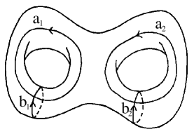
Here’s a schematic of the curves that are hard to lift (which another mathematician used to prove another thing [this whole post should show you that the mathematical community is tight]):

This curve in the surface goes around one part of the surface 4 times, and then heads over to a different part and circles that.  This schematic is a flattened pair of pants, which we've seen before (so the surface keeps going, attached to this thing at three different boundary components)

This curve in the surface goes around one part of the surface 4 times, and then heads over to a different part and circles that. This schematic is a flattened pair of pants, which we’ve seen before (so the surface keeps going, attached to this thing at three different boundary components).  I did not make this picture it is clearly from Jonah’s paper, page 4.

So that’s the story… for now!  From Liverpool (Peter Scott) to Rutgers in New Jersey (Priyam) to Urbana/Champaign in Illinois (Gupta and Kapovitch) to Boston (Jonah), with some quick nods to a ton of other places (see all of their references in their papers).  And the story keeps going.  For instance, if you have a lower bound in terms of length of a curve, you automatically get a lower bound in terms of the number of times it intersects itself (K\sqrt{i(g,g)}\leq \ell(g), same mathematician who came up with the curves).  So an open question is: can you get an upper bound in terms of self-intersection number, not length?

Introduction to the curve complex

21 Jan

This isn’t actually what I’m focusing on, but my friend Matt does his research with this thing.  I think it’s pretty cool so I’ll try to explain what it is.  P.S. I signed up for a class called “Explaining Science” this semester so hopefully my exposition will get clearer.  Or I just need to write more math posts and they will get better.

I’m going to chat with you about the curve complex, so first, let’s think about curves.

simple closed curve on a surface is a big ol’ loop (closed) that doesn’t cross itself (simple).  You can think of these as made of stretchy pieces of string.  Two curves are homotopic if you can push the string from one curve to form the other curve, without jumping across holes.

Red curves are homotopic to each other; blue curve is not

Red curves are homotopic to each other; blue curve is not

So for our example, no matter how you move it, the blue string won’t ever look like either of the red ones, because it’s “stuck” on the big hole in the middle, and no matter how you manipulate it, it has to get around that hole by going to the left half of the torus.  Versus the two red curves are homotopic, because you could suck in that big alien arm from the top red curve, and the little thumb wrapping around the bottom, and then you’d look like the bottom red loop.  We say the red curves are both representatives of the same homotopy class.

At first, it might be tempting to think there’s only two homotopy classes of loops on the torus: red ones, and blue ones.  But then you get green ones:

Green curve not homotopic to either the blue or red ones

Green curve not homotopic to either the blue or red ones

Our green guy wraps around the horizontal axis of our torus once, but it wraps around the vertical way four times.  It totally can’t be manipulated to look like either the red or the blue curves.  [Aside: knot theorists could call this a (4,1) torus knot, for obvious reasons, but since one of the numbers is a 1, the knot is trivial.  E.g. the green curve is just a loop if you took away the torus.  But if it was, say, a (4,2) knot, then it wouldn’t be trivial if you took away the torus.]

My point was this: there’s a whole bunch of homotopy classes of simple closed curves on this very simple surface.  And on any surface, there’s gonna be a whole bunch of homotopy classes of simple closed curves. (In fact, infinitely many.)

Instead of looking at the surface, we can look at those curves and talk about them.  But it’s pretty impossible to just look at a list of curves and say things about it, just like it’s way hard to look at a list of roads and figure out the best way to get from A to B.  What we need is a road map to show how these homotopy classes interact with each other.  And that road map is our curve complex.

So let’s make this map.  For each homotopy class, we form a vertex (like a city).  So in our example, we’re holding three vertices, say R, G, and B.  Then we draw an edge between vertices (like a road between cities) if the homotopy classes have some representatives that don’t intersect.

In our case, no matter how you draw them, all three of our curves intersect.  So they’re just three disjoint vertices in our curve complex.

Here’s a quick example of curves that do have disjoint representatives (image found here):

Disjoint curves

Here, the curves are disjoint, so in the curve complex, there’s an edge in between them.  Anytime we have classes that have representatives that are pairwise disjoint, we add an n-simplex.  So if we had three curves A,B,C so that A and B had pairwise disjoint representatives, B and C had pairwise disjoint representatives, etc., we’d have a triangle in our complex.  Note that these are representatives, so even if the B curve that is disjoint from A intersects C, we’re OK if there’s another curve homotopic to that B curve which is disjoint from C.

So this is the object that my friend Matt thinks about.  There’s a couple cool things to say about it, and I’ll do another post later about this paper I read, but here’s a few goodies:

The curve complex is locally infinite.  So if you’re standing in one city, and you look around, there are infinitely many roads heading out to other cities.  Another way of saying this is that there are infinitely many vertices that are distance 1 away from your vertex.

It’s “hard” to find curves far away from each other. If I give you a curve on a surface, you can probably draw a disjoint nontrivial curve; there’s so many distance 1 away.   In order for two curves to be distance two apart, they have to intersect, and there has to be a third curve disjoint from both of them.  In our picture above, a_1, b_1 
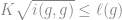
intersect, and both are disjoint from a_2, so that’s okay too.

So for two curves to be bigger than distance 2 apart, there can’t be a third curve disjoint from both of them.  That means that if you had scissors and cut along one curve, and then cut all along the other, you’d end up with a pile of discs (so any curve disjoint from the first two would be trivial).  Another way is saying that these guys have to fill the surface.

We just did distance 1, 2, 3.  It gets harder from there.

But the curve complex has infinite diameter.  I don’t know this well enough to explain it here.  But it’s true: there are roads that have infinitely many cities hanging out on them in our map.

This seems like enough for now.  Curve complexes are pretty hip, and the paper I read was just submitted in October by Joan Birman and William Menasco.  This whole post is in the first paragraph of that paper, so I referred to this talk by Moon Duchin while writing.  There’s a standard way to cite references in math blog posts, just like people standardly write recipes at the end of baking blog posts.  I’ll get the hang of it.  I put in the reference for the second picture by it, but the first picture is an MS Painted version of this picture by Paul Bourke.  

Okay!  Math blog post 2, done!